Human Heart (Visium, a single slice)

import numpy as np
import pandas as pd
import pathlib
import matplotlib.pyplot as plt
import matplotlib as mpl
import seaborn as sns
import scanpy as sc

import sys
sys.path.append('../src')
from utils import *

import warnings
warnings.filterwarnings('ignore')

Preprocessing scRNA-ref

Ideally, the scRNAseq reference should from the exact same tissue that contains all the celltypes you expect to find in ST spots.

We will use a human heart snRNA-seq atlas as reference dataset, the raw dataset in h5ad format (global_raw.h5ad) is available in here.

Conveniently, we provided the pre-pocessed scRNA-ref (Ckpts_scRefs/Heart_D2/Ref_Heart_sanger_D2.h5ad) as well as other relevent materials involved in the following example in here, so you can skip this part

ad_sc = sc.read('global_raw.h5ad')

ad_sc = ad_sc[ad_sc.obs['cell_type']!='doublets']
ad_sc = ad_sc[ad_sc.obs['cell_type']!='NotAssigned']
ad_sc = ad_sc[ad_sc.obs['cell_type']!='Mesothelial']
ad_sc = ad_sc[ad_sc.obs['cell_source']=='Sanger-Nuclei']

cell_type_column = 'cell_type'

sc.pp.filter_cells(ad_sc, min_counts=500)
sc.pp.filter_cells(ad_sc, max_counts=20000)
sc.pp.filter_genes(ad_sc, min_cells=5)
ad_sc = ad_sc[:,~np.array([_.startswith('MT-') for _ in ad_sc.var.index])]
ad_sc = ad_sc[:,~np.array([_.startswith('mt-') for _ in ad_sc.var.index])]

ad_sc = ad_sc[ad_sc.obs['donor']=='D2'].copy() # reduce batch effect among doners
ad_sc = ad_sc[ad_sc.obs.index.isin(ad_sc.obs.groupby('cell_type').apply(
    lambda x: x.sample(frac=3000/x.shape[0],replace=False) if x.shape[0]>3000 else x).reset_index(level=0,drop=True).index)].copy()

ad_sc.X.max(),ad_sc.shape

(6511.0, (17841, 27462))

sns.set_context('paper',font_scale=1.6)
fig, axs = plt.subplots(1, 1, figsize=(10, 10))
sc.pl.umap(
    ad_sc, color=cell_type_column, size=15, frameon=False, show=False, ax=axs,legend_loc='on data'
)
plt.tight_layout()

if ad_sc.X.max()<20:
    ad_sc.X = np.exp(ad_sc.X)-1
plt.hist(ad_sc.X.sum(1),bins=100)
plt.show()

ad_sc.raw = ad_sc.copy()
sc.pp.normalize_total(ad_sc,target_sum=2000)

sc.pp.highly_variable_genes(ad_sc, flavor='seurat_v3',n_top_genes=1000)
sc.tl.rank_genes_groups(ad_sc, groupby=cell_type_column, method='wilcoxon')
markers_df = pd.DataFrame(ad_sc.uns["rank_genes_groups"]["names"]).iloc[0:100, :]
markers = list(np.unique(markers_df.melt().value.values))
markers = list(set(ad_sc.var.loc[ad_sc.var['highly_variable']==1].index)|set(markers)) # highly variable genes + cell type marker genes

ligand_recept = list(set(pd.read_csv('../extdata/ligand_receptors.txt',sep='\t').melt()['value'].values))
# if scRNA-seq reference is from human tissue, run following code to make gene name consistent
ligand_recept = [_.upper() for _ in ligand_recept]
add_genes = 'DCN GSN PDGFRA\
RGS5 ABCC9 KCNJ8\
MYH11 TAGLN ACTA2\
GPAM FASN LEP\
MSLN WT1 BNC1\
VWF PECAM1 CDH5\
CD14 C1QA CD68\
CD8A IL7R CD40LG\
NPPA MYL7 MYL4\
MYH7 MYL2 FHL2\
DLC1 EBF1 SOX5\
FHL1 CNN1 MYH9\
CRYAB NDUFA4 COX7C\
PCDH7 FHL2 MYH7\
PRELID2 GRXCR2 AC107068.2\
MYH6 NPPA MYL4\
CNN1 MYH9 DUSP27\
CKM COX41L NDUFA4\
DLC1 PLA2GS MAML2\
HAMP SLIT3 ALDH1A2\
POSTN TNC FAP\
SCN7A BMPER ACSM1\
FBLN2 PCOLCE2 LINC01133\
CD36 EGFLAM FTL1\
CFH ID4 KCNT2\
PTX3 OSMR IL6ST\
DCN PTX3 C1QA\
NOTCH1 NOTCH2 NOTCH3 NOTCH4 DLL1 DLL4 JAG1 JAG2\
CDH5 SEMA3G ACKR1 MYH11'.split()+['TNNT2','PLN','MYH7','MYL2','IRX3','IRX5','MASP1'] # some important genes that we interested

markers = markers+add_genes+ligand_recept
len(markers)

WARNING: It seems you use rank_genes_groups on the raw count data. Please logarithmize your data before calling rank_genes_groups.

2447

ad_sc.var.loc[ad_sc.var.index.isin(markers),'Marker'] = True
ad_sc.var['Marker'] = ad_sc.var['Marker'].fillna(False)
ad_sc.var['highly_variable'] = ad_sc.var['Marker']

sc.pp.log1p(ad_sc)
sc.pp.pca(ad_sc,svd_solver='arpack', n_comps=30, use_highly_variable=True)

ad_sc.X.max()

7.1928005

sc.pp.neighbors(ad_sc, metric='cosine', n_neighbors=30, n_pcs = 30)
sc.tl.umap(ad_sc, min_dist = 0.5, spread = 1, maxiter=60)

fig, axs = plt.subplots(1, 1, figsize=(10, 10))
sc.pl.umap(
    ad_sc, color=cell_type_column, size=15, frameon=False, show=False, ax=axs,legend_loc='on data'
)
plt.tight_layout()

fig, axs = plt.subplots(1, 1, figsize=(10, 10))
sc.pl.umap(
    ad_sc, color="cell_states", size=10, frameon=False, show=False, ax=axs,legend_loc='on data'
)
plt.tight_layout()

#ad_sc.write('../Ckpts_scRefs/Heart_D2/Ref_Heart_sanger_D2.h5ad')

Learning the gene expression distribution of scRNA-seq reference using score-based model

We use four GPUs to train scRNA-seq reference in parallel.

python ./src/Train_scRef.py \
--ckpt_path ./Ckpts_scRefs/Heart_D2 \
--scRef ./Ckpts_scRefs/Heart_D2/Ref_Heart_sanger_D2.h5ad \
--cell_class_column cell_type \
--gpus 0,1,2,3 \
--sigma_begin 50 --sigma_end 0.002 --step_lr 3e-7

The checkpoints and sampled psuedo-cells will be saved in ./Ckpts_scRefs/Heart_D2, e.g, model_5000.pt, model_5000.h5ad

Due to the low sequencing depth (~2000 UMIs per cell) of this scRNA-seq reference, we changed the default parameters of sigma_begin, sigma_end and step_lr

Conveniently, we provided the pre-trained checkpoint (Ckpts_scRefs/Heart_D2/model_5000.pt) in here, so you can skip this part

Run SpatialScope

Step1: Nuclei segmentation

python ./src/Nuclei_Segmentation.py --tissue heart --out_dir  ./output  --ST_Data ./demo_data/V1_Human_Heart_spatial.h5ad --Img_Data  ./demo_data/V1_Human_Heart_image.tif

Step2: Cell type identification

python ./src/Cell_Type_Identification.py --tissue heart --out_dir  ./output  --ST_Data ./output/heart/sp_adata_ns.h5ad --SC_Data ./Ckpts_scRefs/Heart_D2/Ref_Heart_sanger_D2.h5ad --cell_class_column cell_type

Step3: Gene expression decomposition

Limited by GPU memory, we can only handle at most about 1000 spots in 4 GPUs at a time, so we decompose 1000 spots at a time.

If you are only interested in the ROI region shown in the main text, you can perform gene expression decomposition on this ROI region only for the sake of time

python ./src/Decomposition.py --tissue heart --out_dir  ./output --SC_Data ./Ckpts_scRefs/Heart_D2/Ref_Heart_sanger_D2.h5ad --cell_class_column cell_type  --ckpt_path ./Ckpts_scRefs/Heart_D2/model_5000.pt --spot_range 0,1000 --gpu 0,1,2,3

python ./src/Decomposition.py --tissue heart --out_dir  ./output --SC_Data ./Ckpts_scRefs/Heart_D2/Ref_Heart_sanger_D2.h5ad --cell_class_column cell_type  --ckpt_path ./Ckpts_scRefs/Heart_D2/model_5000.pt --spot_range 1000,2000 --gpu 0,1,2,3

python ./src/Decomposition.py --tissue heart --out_dir  ./output --SC_Data ./Ckpts_scRefs/Heart_D2/Ref_Heart_sanger_D2.h5ad --cell_class_column cell_type  --ckpt_path ./Ckpts_scRefs/Heart_D2/model_5000.pt --spot_range 2000,3000 --gpu 0,1,2,3

python ./src/Decomposition.py --tissue heart --out_dir  ./output --SC_Data ./Ckpts_scRefs/Heart_D2/Ref_Heart_sanger_D2.h5ad --cell_class_column cell_type  --ckpt_path ./Ckpts_scRefs/Heart_D2/model_5000.pt --spot_range 3000,4000 --gpu 0,1,2,3

python ./src/Decomposition.py --tissue heart --out_dir  ./output --SC_Data ./Ckpts_scRefs/Heart_D2/Ref_Heart_sanger_D2.h5ad --cell_class_column cell_type  --ckpt_path ./Ckpts_scRefs/Heart_D2/model_5000.pt --spot_range 4000,4220 --gpu 0,1,2,3

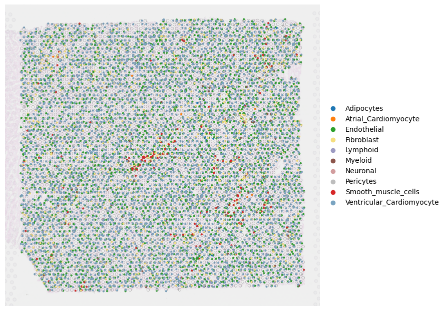
Cell type identification result at single-cell resolution for the whole slice (Fig a)

ad_sc = sc.read('../Ckpts_scRefs/Heart_D2/Ref_Heart_sanger_D2.h5ad')
ad_sp = sc.read('../output/heart/sp_adata.h5ad')

cell_locations will be added to .uns after Step 1 (nuclei segmention)

ad_sp.uns['cell_locations'].head()

	x	y	spot_index	cell_index	cell_nums	discrete_label	discrete_label_ct
0	9850.322581	8497.774194	AAACAAGTATCTCCCA-1	AAACAAGTATCTCCCA-1_0	3	2	Endothelial
1	9834.727626	8509.268482	AAACAAGTATCTCCCA-1	AAACAAGTATCTCCCA-1_1	3	9	Ventricular_Cardiomyocyte
2	9831.670886	8492.797468	AAACAAGTATCTCCCA-1	AAACAAGTATCTCCCA-1_2	3	9	Ventricular_Cardiomyocyte
3	4112.213235	9584.580882	AAACACCAATAACTGC-1	AAACACCAATAACTGC-1_0	4	3	Fibroblast
4	4074.684874	9610.348739	AAACACCAATAACTGC-1	AAACACCAATAACTGC-1_1	4	2	Endothelial

color_dict = {'Adipocytes': '#1f77b4',
 'Atrial_Cardiomyocyte': '#ff7f0e',
 'Endothelial': '#2ca02c',
 'Fibroblast': '#F5DE7E',
 'Lymphoid': '#9D9BC2',
 'Myeloid': '#8c564b',
 'Neuronal': '#D29D9E',
 'Pericytes': '#BDBDBD',
 'Smooth_muscle_cells': '#d62728',
 'Ventricular_Cardiomyocyte': '#7AA4C1'}

fig, ax = plt.subplots(1,1,figsize=(12, 8),dpi=100)
PlotVisiumCells(ad_sp,"discrete_label_ct",size=0.7,alpha_img=0.2,lw=0.3,palette=color_dict,ax=ax)

/import/home/jxiaoae/spatial/SpatialScope-Beta/demos/../src/utils.py:74: FutureWarning: X.dtype being converted to np.float32 from float64. In the next version of anndata (0.9) conversion will not be automatic. Pass dtype explicitly to avoid this warning. Pass `AnnData(X, dtype=X.dtype, ...)` to get the future behavour.
  test = sc.AnnData(np.zeros(merged_df.shape), obs=merged_df)
/home/jxiaoae/.conda/envs/SpatialScope/lib/python3.9/site-packages/anndata/_core/anndata.py:121: ImplicitModificationWarning: Transforming to str index.
  warnings.warn("Transforming to str index.", ImplicitModificationWarning)

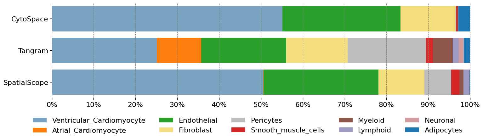
Inferred cell type compositions (Fig b)

p2_res = ad_sp.uns['cell_locations']
ss = pd.DataFrame(p2_res.discrete_label_ct.value_counts()/p2_res.shape[0])
ss.columns = ['SpatialScope']


alignres_cytospace = pd.read_csv('/home/share/xiaojs/spatial/sour_sep/heart/res/cytospace/D2/cytospace_results/assigned_locations.csv')
cs = pd.DataFrame(alignres_cytospace['CellType'].value_counts()/alignres_cytospace.shape[0])
cs.columns = ['CytoSpace']

tg = pd.read_csv('/home/share/xiaojs/spatial/sour_sep/heart/res/Tangram_P2_D2Ref_nu10.csv',index_col=0)
tg = pd.DataFrame(tg['cluster'].value_counts()/tg.shape[0])
tg.columns = ['Tangram']

df_res = ss.merge(tg,left_index=True,right_index=True,how='outer').merge(cs,left_index=True,right_index=True,how='outer')

df_res = df_res.fillna(0).T

df_res

	Adipocytes	Atrial_Cardiomyocyte	Endothelial	Fibroblast	Lymphoid	Myeloid	Neuronal	Pericytes	Smooth_muscle_cells	Ventricular_Cardiomyocyte
SpatialScope	0.001846	0.000646	0.275337	0.109378	0.013661	0.009692	0.000738	0.063965	0.019476	0.505261
Tangram	0.014879	0.106452	0.203436	0.146896	0.014473	0.047207	0.012444	0.187204	0.016367	0.250642
CytoSpace	0.027632	0.000000	0.282416	0.131340	0.002153	0.000000	0.000000	0.001914	0.003230	0.551316

# variables
plot_columns = ['Ventricular_Cardiomyocyte','Atrial_Cardiomyocyte',
 'Endothelial',
 'Fibroblast',
 'Pericytes',
 'Smooth_muscle_cells',
 'Myeloid',
 'Lymphoid',
 'Neuronal',
 'Adipocytes']
plot_colors = [color_dict[_] for _ in plot_columns]

labels = plot_columns#df_res.columns
colors = plot_colors#['#1D2F6F', '#8390FA', '#6EAF46', '#FAC748']
title = 'Video Game Sales By Platform and Region\n'
subtitle = 'Proportion of Games Sold by Region'
def plot_stackedbar_p(df, labels, colors, title, subtitle):
    fields = labels#df.columns.tolist()

    # figure and axis
    sns.set_context('paper',font_scale=1.8)
    fig, ax = plt.subplots(1, figsize=(18, 4),dpi=100)
# plot bars
    left = len(df) * [0]
    for idx, name in enumerate(fields):
        plt.barh(df.index, df[name], left = left, color=colors[idx])
        left = left + df[name]
# legend
    plt.legend(labels, bbox_to_anchor=([.95, -0.14, 0, 0]), ncol=5, frameon=False)
# remove spines
    ax.spines['right'].set_visible(False)
    ax.spines['left'].set_visible(False)
    ax.spines['top'].set_visible(False)
    ax.spines['bottom'].set_visible(False)
# format x ticks
    xticks = np.arange(0,1.1,0.1)
    xlabels = ['{}%'.format(i) for i in np.arange(0,101,10)]
    plt.xticks(xticks, xlabels)
# adjust limits and draw grid lines
    plt.ylim(-0.5, ax.get_yticks()[-1] + 0.5)
    ax.xaxis.grid(color='gray', linestyle='dashed')
plt.show()

plot_stackedbar_p(df_res, labels, colors, title, subtitle)

UMAP of single cell reference data (Fig c)

scRef and sampled pseudo-cells

sampled_cells = sc.read('../Ckpts_scRefs/Heart_D2/model_5000.h5ad') # 2K cells sampled from the learned gene expression distribution of scRef
cell_type_key='cell_type'
sns.set_context('paper',font_scale=1.5)
adata_all = PlotSampledData(sampled_cells,ad_sc,cell_type_key,palette=color_dict)

/home/jxiaoae/.conda/envs/SpatialScope/lib/python3.9/site-packages/anndata/_core/merge.py:942: UserWarning: Only some AnnData objects have `.raw` attribute, not concatenating `.raw` attributes.
  warn(
/home/jxiaoae/.conda/envs/SpatialScope/lib/python3.9/site-packages/anndata/_core/anndata.py:1785: FutureWarning: X.dtype being converted to np.float32 from float64. In the next version of anndata (0.9) conversion will not be automatic. Pass dtype explicitly to avoid this warning. Pass `AnnData(X, dtype=X.dtype, ...)` to get the future behavour.
  [AnnData(sparse.csr_matrix(a.shape), obs=a.obs) for a in all_adatas],

AnnData object with n_obs × n_vars = 19369 × 2195
    obs: 'NRP', 'age_group', 'cell_source', 'cell_type', 'donor', 'gender', 'n_counts', 'n_genes', 'percent_mito', 'percent_ribo', 'region', 'sample', 'scrublet_score', 'source', 'type', 'version', 'cell_states', 'Used', 'cell type', 'batch'
    var: 'gene_ids-Harvard-Nuclei', 'feature_types-Harvard-Nuclei', 'gene_ids-Sanger-Nuclei', 'feature_types-Sanger-Nuclei', 'gene_ids-Sanger-Cells', 'feature_types-Sanger-Cells', 'gene_ids-Sanger-CD45', 'feature_types-Sanger-CD45', 'n_cells', 'highly_variable', 'highly_variable_rank', 'means', 'variances', 'variances_norm', 'Marker', 'mean-0', 'std-0', 'mean-1', 'std-1'
    uns: 'neighbors', 'umap', 'cell_type_colors'
    obsm: 'X_pca', 'X_umap'
    varm: 'PCs'
    obsp: 'distances', 'connectivities'

Cell type identification result at single-cell resolution in ROI (Fig d)

import squidpy as sq

image = plt.imread('../demo_data/V1_Human_Heart_image.tif')
img = sq.im.ImageContainer(image)

/home/jxiaoae/.conda/envs/SpatialScope/lib/python3.9/site-packages/PIL/Image.py:3011: DecompressionBombWarning: Image size (177742224 pixels) exceeds limit of 89478485 pixels, could be decompression bomb DOS attack.
  warnings.warn(

crop = img.crop_corner(0, 0)
crop.show(channelwise=True,layer='image')

crop

ImageContainer object with 1 layer:

image: y (13332), x (13332), z (1), channels (3)

inset_x = int(img.shape[0]*(4.1/10)) # column
inset_y = int(img.shape[1]*(4.6/10)) # row
inset_sx = int(img.shape[0]*(2/10))
inset_sy = int(img.shape[1]*(1.6/10))

ad_sp_crop = ad_sp[
    (ad_sp.obsm["spatial"][:, 0] > inset_x) & (ad_sp.obsm["spatial"][:, 1] > inset_y)
    & (ad_sp.obsm["spatial"][:, 0] < inset_x+inset_sx) & (ad_sp.obsm["spatial"][:, 1] < inset_y+inset_sy), :
].copy()

ad_sp_crop.uns['cell_locations'] = ad_sp_crop.uns['cell_locations'].loc[ad_sp_crop.uns['cell_locations'].spot_index.isin(ad_sp_crop.obs.index)].reset_index(drop=True)

fig, ax = plt.subplots(1,1,figsize=(12, 8),dpi=100)
PlotVisiumCells(ad_sp_crop,"discrete_label_ct",size=0.3,alpha_img=0.3,lw=0.8,palette=color_dict,ax=ax)

/import/home/jxiaoae/spatial/SpatialScope-Beta/demos/../src/utils.py:77: FutureWarning: X.dtype being converted to np.float32 from float64. In the next version of anndata (0.9) conversion will not be automatic. Pass dtype explicitly to avoid this warning. Pass `AnnData(X, dtype=X.dtype, ...)` to get the future behavour.
  test = sc.AnnData(np.zeros(merged_df.shape), obs=merged_df)
/home/jxiaoae/.conda/envs/SpatialScope/lib/python3.9/site-packages/anndata/_core/anndata.py:121: ImplicitModificationWarning: Transforming to str index.
  warnings.warn("Transforming to str index.", ImplicitModificationWarning)

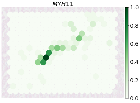
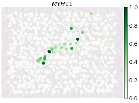
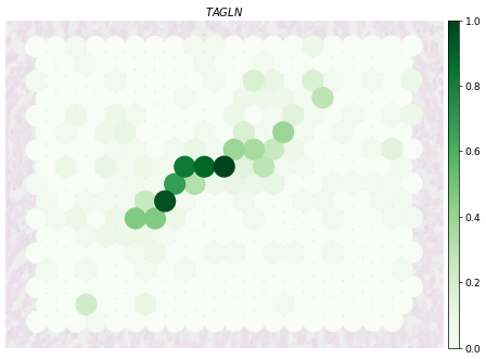
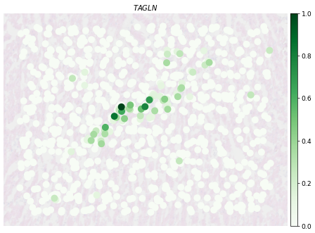
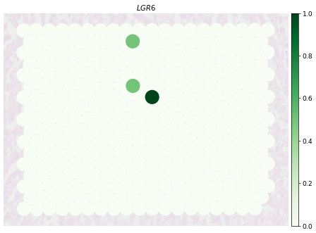
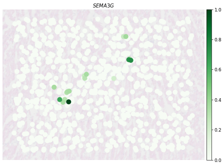
Expression of SMC and EC marker genes (Fig e)

We start by concatenating all the generated_cells_spotX-X.h5ad together.

If you are only interested in this ROI region, you can perform gene expression decomposition on this ROI region only for the sake of time

ad_scsts_list = []
ad_scsts_list.append(sc.read('../output/heart/generated_cells_spot0_1000.h5ad'))
ad_scsts_list.append(sc.read('../output/heart/generated_cells_spot1000_2000.h5ad'))
ad_scsts_list.append(sc.read('../output/heart/generated_cells_spot2000_3000.h5ad'))
ad_scsts_list.append(sc.read('../output/heart/generated_cells_spot3000_4000.h5ad'))
ad_scsts_list.append(sc.read('../output/heart/generated_cells_spot4000_4220.h5ad'))

ad_scsts = ad_scsts_list[0].concatenate(
        ad_scsts_list[1:],
        batch_key="_",
        uns_merge="unique",
        index_unique=None
        )

/home/jxiaoae/.conda/envs/SpatialScope/lib/python3.9/site-packages/anndata/_core/anndata.py:1785: FutureWarning: X.dtype being converted to np.float32 from float64. In the next version of anndata (0.9) conversion will not be automatic. Pass dtype explicitly to avoid this warning. Pass `AnnData(X, dtype=X.dtype, ...)` to get the future behavour.
  [AnnData(sparse.csr_matrix(a.shape), obs=a.obs) for a in all_adatas],

ad_scst_crop = = ad_scsts[ad_scsts.obs['spot_index'].isin(ad_sp_crop.obs.index)]
# If you are only interested in this ROI region, you can perform gene expression decomposition on this ROI region only for the sake of time

ad_scst_crop.uns = ad_sp_crop.uns

ad_scst_crop

AnnData object with n_obs × n_vars = 873 × 2195
    obs: 'x', 'y', 'spot_index', 'cell_index', 'cell_nums', 'discrete_label', 'discrete_label_ct'
    uns: 'cell_locations', 'spatial', 'log1p'

ad_scst_crop.write('../demo_data/human_heart_ROI_generated_cells.h5ad')

ad_scst_crop.obs.head()

	x	y	spot_index	cell_index	cell_nums	discrete_label	discrete_label_ct
64	7384.721649	7905.711340	AAACTGCTGGCTCCAA-1	AAACTGCTGGCTCCAA-1_0	1	9	Ventricular_Cardiomyocyte
115	7521.504808	8177.100962	AAATACCTATAAGCAT-1	AAATACCTATAAGCAT-1_0	4	9	Ventricular_Cardiomyocyte
116	7567.760000	8129.320000	AAATACCTATAAGCAT-1	AAATACCTATAAGCAT-1_1	4	3	Fibroblast
117	7553.000000	8118.000000	AAATACCTATAAGCAT-1	AAATACCTATAAGCAT-1_2	4	2	Endothelial
118	7555.917355	8140.165289	AAATACCTATAAGCAT-1	AAATACCTATAAGCAT-1_3	4	9	Ventricular_Cardiomyocyte

ad_sp_crop.X.max(),ad_scst_crop.X.max()

(420.0001, 1381.0935)

fig, ax = plt.subplots(1, 1, figsize=(12, 8),dpi=50)
PlotVisiumGene(ad_sp_crop,'MYH11',ax=ax,size=1.7,alpha_img=0.2,palette='Greens')

fig, ax = plt.subplots(1, 1, figsize=(12, 8),dpi=50)
PlotVisiumGene(ad_scst_crop,'MYH11',ax=ax,size=2.5,alpha_img=0.2,palette='Greens')

fig, ax = plt.subplots(1, 1, figsize=(12, 8),dpi=50)
PlotVisiumGene(ad_sp_crop,'TAGLN',ax=ax,size=1.7,alpha_img=0.2,palette='Greens')

fig, ax = plt.subplots(1, 1, figsize=(12, 8),dpi=50)
PlotVisiumGene(ad_scst_crop,'TAGLN',ax=ax,size=2.5,alpha_img=0.2,palette='Greens')

fig, ax = plt.subplots(1, 1, figsize=(12, 8),dpi=50)
PlotVisiumGene(ad_sp_crop,'LGR6',ax=ax,size=1.7,alpha_img=0.2,palette='Greens')

fig, ax = plt.subplots(1, 1, figsize=(12, 8),dpi=50)
PlotVisiumGene(ad_scst_crop,'LGR6',ax=ax,size=2.5,alpha_img=0.2,palette='Greens')

fig, ax = plt.subplots(1, 1, figsize=(12, 8),dpi=50)
PlotVisiumGene(ad_sp_crop,'VWF',ax=ax,size=1.7,alpha_img=0.2,palette='Greens')

fig, ax = plt.subplots(1, 1, figsize=(12, 8),dpi=50)
PlotVisiumGene(ad_scst_crop,'VWF',ax=ax,size=2.5,alpha_img=0.2,palette='Greens')

fig, ax = plt.subplots(1, 1, figsize=(12, 8),dpi=50)
PlotVisiumGene(ad_sp_crop,'SEMA3G',ax=ax,size=1.7,alpha_img=0.2,palette='Greens')

fig, ax = plt.subplots(1, 1, figsize=(12, 8),dpi=50)
PlotVisiumGene(ad_scst_crop,'SEMA3G',ax=ax,size=2.5,alpha_img=0.2,palette='Greens')

SpatialScope inferred SMCs (Fig f)

ad_scst_crop = sc.read('../demo_data/human_heart_ROI_generated_cells.h5ad')

smscells_gx = ad_scst_crop[ad_scst_crop.obs['discrete_label_ct']=='Smooth_muscle_cells'].copy()
smscells_gx.obs['cell_type'] = 'Generated_SMC_Cells'
smscells_gx.obs['cell_states'] = 'Generated_SMC_Cells'
sc.pp.log1p(smscells_gx)

ad_sc = sc.read('../Ckpts_scRefs/Heart_D2/Ref_Heart_sanger_D2.h5ad')
ad_sc = ad_sc[ad_sc.obs['cell_type'].isin(['Endothelial','Smooth_muscle_cells'])]
ad_sc = ad_sc[~ad_sc.obs['cell_states'].isin(['EC4_immune','EC10_CMC-like','EC9_FB-like','EC8_ln'])]
ad_sc = ad_sc[:,ad_sc.var.Marker]
rename_dict = {
    'EC1_cap':'EC_cap',
    'EC3_cap':'EC_cap',
    'EC2_cap':'EC_cap'
}

ad_sc.obs['cell_states'] = ad_sc.obs['cell_states'].map(lambda x:rename_dict[x] if x in rename_dict.keys() else x)

WARNING: adata.X seems to be already log-transformed.

/home/share/xiaojs/software/netMHCpan-4.1/Linux_x86_64/tmp/ipykernel_37314/3122457914.py:16: ImplicitModificationWarning: Trying to modify attribute `.obs` of view, initializing view as actual.
  ad_sc.obs['cell_states'] = ad_sc.obs['cell_states'].map(lambda x:rename_dict[x] if x in rename_dict.keys() else x)

ad_sc.X.max(),smscells_gx.X.max()

(6.9823365, 6.4401555)

ad_sc.uns['log1p']['base'] = None
sc.pp.highly_variable_genes(ad_sc, n_top_genes=500)
sc.tl.pca(ad_sc, n_comps=30, use_highly_variable=True)

pcs = ad_sc.varm['PCs']
smscells_gx.obsm['X_pca'] = (smscells_gx.X - ad_sc.X.mean(0)) @ pcs

adata_all = ad_sc.concatenate(smscells_gx)

adata_all.varm['PCs'] = pcs
adata_all.raw = adata_all
sc.pp.neighbors(adata_all, n_neighbors=20, n_pcs=30)
sc.tl.umap(adata_all, min_dist = 0.5, spread = 1., maxiter = 50)

/home/jxiaoae/.conda/envs/SpatialScope/lib/python3.9/site-packages/anndata/_core/merge.py:942: UserWarning: Only some AnnData objects have `.raw` attribute, not concatenating `.raw` attributes.
  warn(
/home/jxiaoae/.conda/envs/SpatialScope/lib/python3.9/site-packages/anndata/_core/anndata.py:1785: FutureWarning: X.dtype being converted to np.float32 from float64. In the next version of anndata (0.9) conversion will not be automatic. Pass dtype explicitly to avoid this warning. Pass `AnnData(X, dtype=X.dtype, ...)` to get the future behavour.
  [AnnData(sparse.csr_matrix(a.shape), obs=a.obs) for a in all_adatas],
/home/jxiaoae/.conda/envs/SpatialScope/lib/python3.9/site-packages/sklearn/utils/validation.py:727: FutureWarning: np.matrix usage is deprecated in 1.0 and will raise a TypeError in 1.2. Please convert to a numpy array with np.asarray. For more information see: https://numpy.org/doc/stable/reference/generated/numpy.matrix.html
  warnings.warn(

fig, axs = plt.subplots(1, 1, figsize=(11, 10),dpi=100)
plt.rcParams["legend.markerscale"] = 1.3
sns.set_context('paper',font_scale=2.2)
sc.pl.umap(
    adata_all, color="cell_states", size=80, frameon=False, palette='Set1', alpha=0.7, show=False, ax=axs#,legend_loc='on data'
)
plt.tight_layout()

Cellular communications detected from SpatialScope generated single-cell resolution spatial data (Fig g)

ad_scst_crop = sc.read('../demo_data/human_heart_ROI_generated_cells.h5ad')
ad_scst_crop.to_df().T.to_csv('../output/heart/express.txt', sep='\t')
ad_scst_crop.obs.loc[:,['x', 'y']].to_csv('../output/heart/coords.txt', sep='\t', index = False)
ad_scst_crop.obs['discrete_label_ct'].to_csv('../output/heart/cell_type.txt', sep='\t', index = False, header = False)

see Human-Heart-CCell-interaction.ipynb or Human heart cell-cell interaction analysis using Giotto section

Fig h

Figure h was drawn by our first author, a painting lover, Xiaomeng

Representative examples (Fig i)

ad_scst_crop = sc.read('../demo_data/human_heart_ROI_generated_cells.h5ad')

ad_scst_crop

AnnData object with n_obs × n_vars = 873 × 2195
    obs: 'x', 'y', 'spot_index', 'cell_index', 'cell_nums', 'discrete_label', 'discrete_label_ct'
    uns: 'cell_locations', 'log1p', 'spatial'

gene_L,gene_R,celltype_L,celltype_R = 'JAG1','NOTCH3','Endothelial','Smooth_muscle_cells'
L_ct_index = ad_scst_crop.obs['discrete_label_ct'].isin(np.array([celltype_L]))
R_ct_index = ad_scst_crop.obs['discrete_label_ct'].isin(np.array([celltype_R]))

sns.set_context('paper',font_scale=3)
fig, ax = plt.subplots(1,2,figsize=(13, 5),dpi=100)
PlotVisiumGene(ad_scst_crop, gene_L, size=2,alpha_img=0.1,perc=0.0,palette='rocket_r',ax=ax[0],vis_index = np.array(L_ct_index),colorbar_loc=None)
PlotVisiumGene(ad_scst_crop, gene_R, size=2,alpha_img=0.1,perc=0.0,palette='Greens',ax=ax[1],vis_index = np.array(R_ct_index),colorbar_loc=None)
fig.tight_layout(pad=0.03)
plt.show()

gene_L,gene_R,celltype_L,celltype_R = 'DLL4','NOTCH3','Endothelial','Smooth_muscle_cells'
L_ct_index = ad_scst_crop.obs['discrete_label_ct'].isin(np.array([celltype_L]))
R_ct_index = ad_scst_crop.obs['discrete_label_ct'].isin(np.array([celltype_R]))

sns.set_context('paper',font_scale=3)
fig, ax = plt.subplots(1,2,figsize=(13, 5),dpi=100)
PlotVisiumGene(ad_scst_crop, gene_L, size=2,alpha_img=0.1,perc=0.0,palette='rocket_r',ax=ax[0],vis_index = np.array(L_ct_index),colorbar_loc=None)
PlotVisiumGene(ad_scst_crop, gene_R, size=2,alpha_img=0.1,perc=0.0,palette='Greens',ax=ax[1],vis_index = np.array(R_ct_index),colorbar_loc=None)
fig.tight_layout(pad=0.03)
plt.show()

gene_L,gene_R,celltype_L,celltype_R = 'SERPINE2','LRP1','Endothelial','Smooth_muscle_cells'
L_ct_index = ad_scst_crop.obs['discrete_label_ct'].isin(np.array([celltype_L]))
R_ct_index = ad_scst_crop.obs['discrete_label_ct'].isin(np.array([celltype_R]))

sns.set_context('paper',font_scale=3)
fig, ax = plt.subplots(1,2,figsize=(13, 5),dpi=100)
PlotVisiumGene(ad_scst_crop, gene_L, size=2,alpha_img=0.1,perc=0.0,palette='rocket_r',ax=ax[0],vis_index = np.array(L_ct_index),colorbar_loc=None)
PlotVisiumGene(ad_scst_crop, gene_R, size=2,alpha_img=0.1,perc=0.0,palette='Greens',ax=ax[1],vis_index = np.array(R_ct_index),colorbar_loc=None)
fig.tight_layout(pad=0.03)
plt.show()