Human heart cell-cell interaction analysis using Giotto
[145]:
library(Giotto)
library(data.table)
[168]:
# tissue = HComD2
path_to_matrix = '../output/heart/express.txt'
path_to_locations = '../output/heart/coords.txt'
path_to_celltype = '../output/heart/cell_type.txt'
my_cell_metadata = read.table(path_to_celltype)
[169]:
my_instructions = createGiottoInstructions(python_path='/home/xwanaf/.conda/envs/rbayes/bin/python')
my_giotto_object = createGiottoObject(raw_exprs = path_to_matrix,
                                      spatial_locs = path_to_locations,
                                      cell_metadata = my_cell_metadata,
                                      instructions = my_instructions)
my_giotto_object@cell_metadata$cell_types <- my_giotto_object@cell_metadata$V1
 external python path provided and will be used
Consider to install these (optional) packages to run all possible Giotto commands for spatial analyses:  MAST smfishHmrf trendsceek SPARK multinet RTriangle FactoMiner
 Giotto does not automatically install all these packages as they are not absolutely required and this reduces the number of dependencies
[4]:
# processing
my_giotto_object <- filterGiotto(gobject = my_giotto_object,
expression_threshold = 0.5,
gene_det_in_min_cells = 20,
min_det_genes_per_cell = 0)
my_giotto_object <- normalizeGiotto(gobject = my_giotto_object)
# dimension reduction
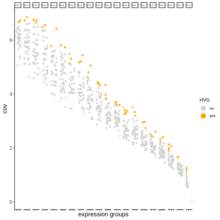
my_giotto_object <- calculateHVG(gobject = my_giotto_object)
my_giotto_object <- runPCA(gobject = my_giotto_object)
my_giotto_object <- runUMAP(my_giotto_object, dimensions_to_use = 1:5)
my_giotto_object <- createNearestNetwork(my_giotto_object)
return_plot = TRUE and return_gobject = TRUE

          plot will not be returned to object, but can still be saved with save_plot = TRUE or manually
hvg  was found in the gene metadata information and will be used to select highly variable genes
Warning message in runPCA_prcomp_irlba(x = t_giotto(expr_values), center = center, :
“ncp >= minimum dimension of x, will be set to minimum dimension of x - 1”
Warning message in (function (A, nv = 5, nu = nv, maxit = 1000, work = nv + 7, reorth = TRUE, :
“You're computing too large a percentage of total singular values, use a standard svd instead.”
Warning message in (function (A, nv = 5, nu = nv, maxit = 1000, work = nv + 7, reorth = TRUE, :
“did not converge--results might be invalid!; try increasing work or maxit”
[5]:
# # annotate
# metadata = pDataDT(my_giotto_object)
# uniq_clusters = length(unique(metadata$leiden_clus))

# clusters_cell_types = paste0('cell ', LETTERS[1:uniq_clusters])
# names(clusters_cell_types) = 1:uniq_clusters

# my_giotto_object = annotateGiotto(gobject = my_giotto_object,
#                               annotation_vector = clusters_cell_types,
#                               cluster_column = 'leiden_clus',
#                               name = 'cell_types')

# create network (required for binSpect methods)
my_giotto_object = createSpatialNetwork(gobject = my_giotto_object, minimum_k = 2)

# identify genes with a spatial coherent expression profile
km_spatialgenes = binSpect(my_giotto_object, bin_method = 'kmeans')
 This is the single parameter version of binSpect
 1. matrix binarization complete

 2. spatial enrichment test completed

 3. (optional) average expression of high expressing cells calculated

 4. (optional) number of high expressing cells calculated
[6]:
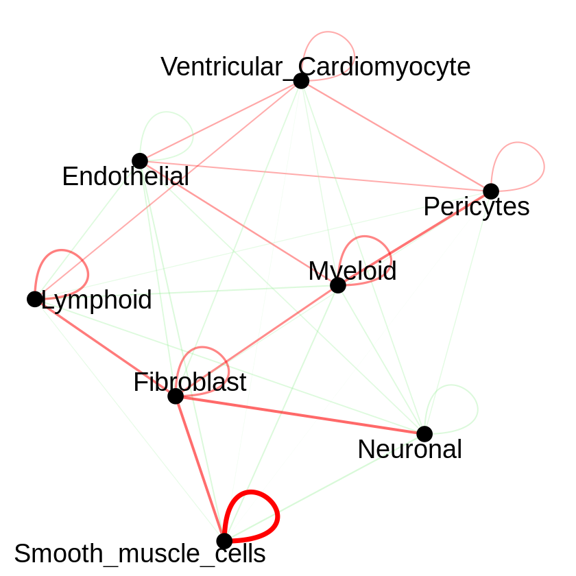
set.seed(seed = 2841)
cell_proximities = cellProximityEnrichment(gobject = my_giotto_object,
                                           cluster_column = 'cell_types',
                                           spatial_network_name = 'Delaunay_network',
                                           adjust_method = 'fdr',
                                           number_of_simulations = 1000)
# network with self-edges
cellProximityNetwork(gobject = my_giotto_object, CPscore = cell_proximities,
                     remove_self_edges = F, self_loop_strength = 0.3,
                     only_show_enrichment_edges = F,
                     rescale_edge_weights = T,
                     node_size = 6, node_text_size=8,
                     edge_weight_range_depletion = c(1, 2),
                     edge_weight_range_enrichment = c(2,5))

[7]:
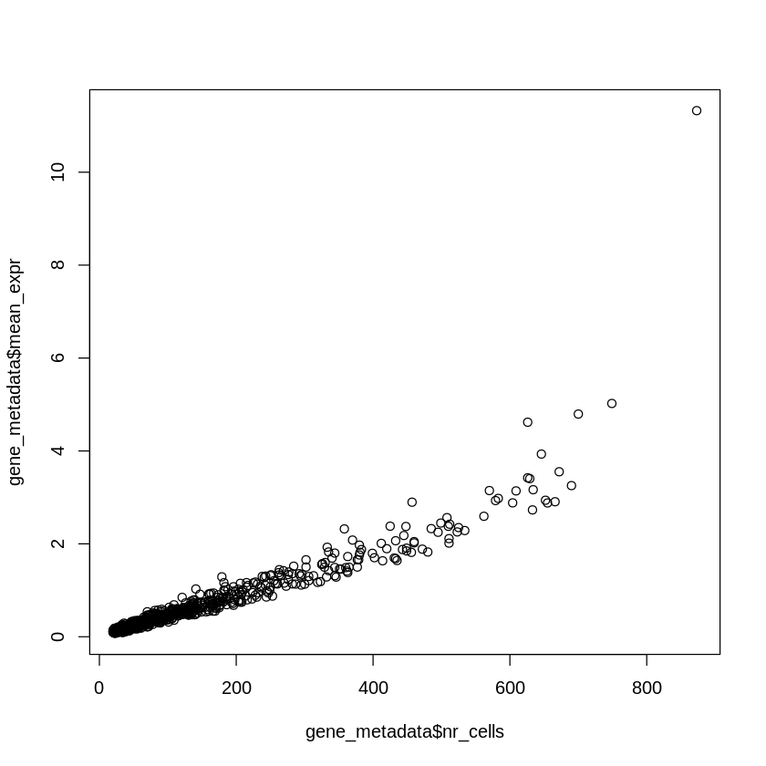
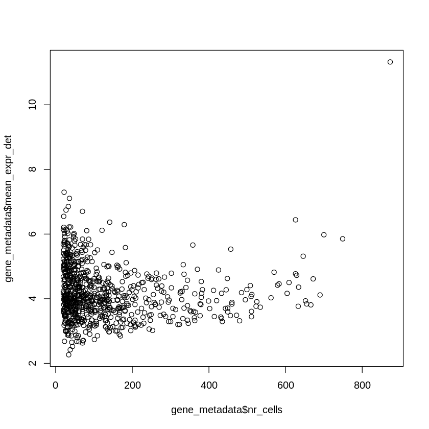
my_giotto_object <- addGeneStatistics(my_giotto_object)
## select top 25th highest expressing genes
gene_metadata = fDataDT(my_giotto_object)
plot(gene_metadata$nr_cells, gene_metadata$mean_expr)
plot(gene_metadata$nr_cells, gene_metadata$mean_expr_det)
quantile(gene_metadata$mean_expr_det)
high_expressed_genes = gene_metadata[mean_expr_det > 4]$gene_ID
## identify genes that are associated with proximity to other cell types
ICGscoresHighGenes = findICG(gobject = my_giotto_object,
selected_genes = high_expressed_genes,
spatial_network_name = 'Delaunay_network',
cluster_column = 'cell_types',
diff_test = 'permutation',
adjust_method = 'fdr',
nr_permutations = 500,
do_parallel = T, cores = 2)
## visualize all genes
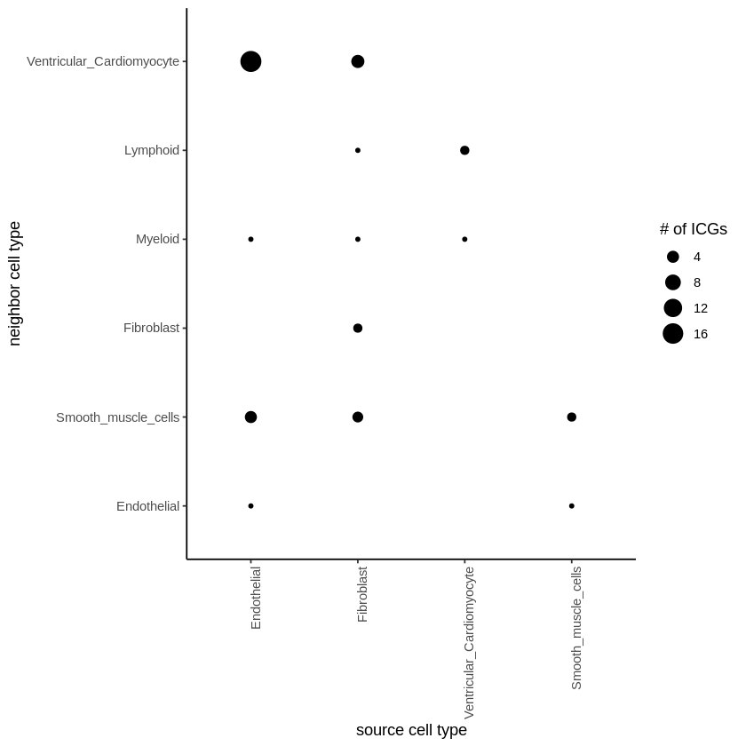
plotCellProximityGenes(my_giotto_object, cpgObject = ICGscoresHighGenes, method = 'dotplot')
## filter genes
ICGscoresFilt = filterICG(ICGscoresHighGenes,
min_cells = 2, min_int_cells = 2, min_fdr = 0.1,
min_spat_diff = 0.1, min_log2_fc = 0.1, min_zscore = 0.0)
# ICGscoresFilt = filterICG(ICGscoresHighGenes,
# min_cells = 2, min_int_cells = 2, min_fdr = 0.1,
# min_spat_diff = 0.1, min_log2_fc = 0.1, min_zscore = 1)
- 0%
- 2.26574402750246
- 25%
- 3.63427153928577
- 50%
- 4.05780871264046
- 75%
- 4.64868220483457
- 100%
- 11.3255376347626

[8]:
# write.csv(ICGscoresHighGenes$CPGscores, '/home/share/xwanaf/sour_sep/newCKPT/MerM/giotto_data/ICGscoresHighGenes.csv', row.names = FALSE)
# write.csv(ICGscoresFilt$CPGscores, '/home/share/xwanaf/sour_sep/newCKPT/MerM/giotto_data/ICGscoresFilt_zscore0.csv', row.names = FALSE)
[ ]:
[9]:
LR_data = data.table::fread(system.file("extdata", "mouse_ligand_receptors.txt", package = 'Giotto'))
LR_data$L_upper = toupper(LR_data$mouseLigand)
LR_data$R_upper = toupper(LR_data$mouseReceptor)
LR_data[, ligand_det := ifelse(L_upper %in% my_giotto_object@gene_ID, T, F)]
LR_data[, receptor_det := ifelse(R_upper %in% my_giotto_object@gene_ID, T, F)]
LR_data_det = LR_data[ligand_det == T & receptor_det == T]
select_ligands = LR_data_det$L_upper
select_receptors = LR_data_det$R_upper
## get statistical significance of gene pair expression changes based on expression ##
expr_only_scores = exprCellCellcom(gobject = my_giotto_object,
cluster_column = 'cell_types',
random_iter = 500,
gene_set_1 = select_ligands,
gene_set_2 = select_receptors)
## get statistical significance of gene pair expression changes upon cell-cell interaction
spatial_all_scores = spatCellCellcom(my_giotto_object,
spatial_network_name = 'Delaunay_network',
cluster_column = 'cell_types',
random_iter = 500,
gene_set_1 = select_ligands,
gene_set_2 = select_receptors,
adjust_method = 'fdr',
do_parallel = T,
cores = 4,
verbose = 'none')
## * plot communication scores ####
## select top LR ##
selected_spat = spatial_all_scores[p.adj <= 0.5 & abs(log2fc) > 0.1 & lig_nr >= 10 & rec_nr >= 10]
data.table::setorder(selected_spat, -PI)
top_LR_ints = unique(selected_spat[order(-abs(PI))]$LR_comb)[1:33]
top_LR_cell_ints = unique(selected_spat[order(-abs(PI))]$LR_cell_comb)[1:33]
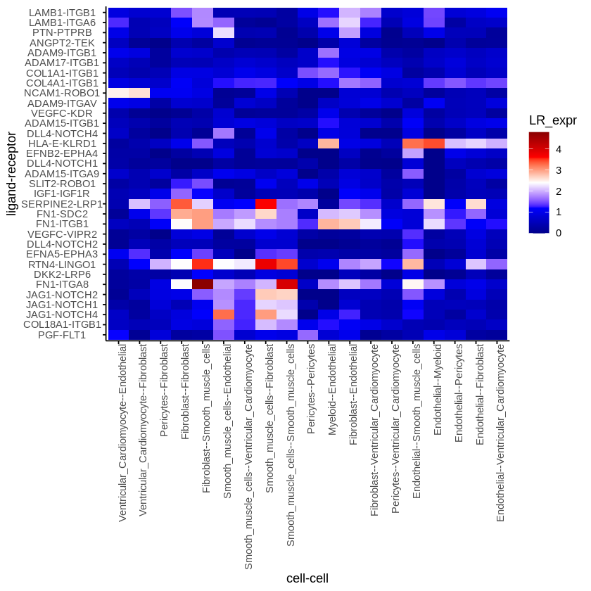
plotCCcomHeatmap(gobject = my_giotto_object,
comScores = spatial_all_scores,
selected_LR = top_LR_ints,
selected_cell_LR = top_LR_cell_ints,
show = 'LR_expr')
simulation  1
simulation  2
simulation  3
simulation  4
simulation  5
simulation  6
simulation  7
simulation  8
simulation  9
simulation  10
simulation  11
simulation  12
simulation  13
simulation  14
simulation  15
simulation  16
simulation  17
simulation  18
simulation  19
simulation  20
simulation  21
simulation  22
simulation  23
simulation  24
simulation  25
simulation  26
simulation  27
simulation  28
simulation  29
simulation  30
simulation  31
simulation  32
simulation  33
simulation  34
simulation  35
simulation  36
simulation  37
simulation  38
simulation  39
simulation  40
simulation  41
simulation  42
simulation  43
simulation  44
simulation  45
simulation  46
simulation  47
simulation  48
simulation  49
simulation  50
simulation  51
simulation  52
simulation  53
simulation  54
simulation  55
simulation  56
simulation  57
simulation  58
simulation  59
simulation  60
simulation  61
simulation  62
simulation  63
simulation  64
simulation  65
simulation  66
simulation  67
simulation  68
simulation  69
simulation  70
simulation  71
simulation  72
simulation  73
simulation  74
simulation  75
simulation  76
simulation  77
simulation  78
simulation  79
simulation  80
simulation  81
simulation  82
simulation  83
simulation  84
simulation  85
simulation  86
simulation  87
simulation  88
simulation  89
simulation  90
simulation  91
simulation  92
simulation  93
simulation  94
simulation  95
simulation  96
simulation  97
simulation  98
simulation  99
simulation  100
simulation  101
simulation  102
simulation  103
simulation  104
simulation  105
simulation  106
simulation  107
simulation  108
simulation  109
simulation  110
simulation  111
simulation  112
simulation  113
simulation  114
simulation  115
simulation  116
simulation  117
simulation  118
simulation  119
simulation  120
simulation  121
simulation  122
simulation  123
simulation  124
simulation  125
simulation  126
simulation  127
simulation  128
simulation  129
simulation  130
simulation  131
simulation  132
simulation  133
simulation  134
simulation  135
simulation  136
simulation  137
simulation  138
simulation  139
simulation  140
simulation  141
simulation  142
simulation  143
simulation  144
simulation  145
simulation  146
simulation  147
simulation  148
simulation  149
simulation  150
simulation  151
simulation  152
simulation  153
simulation  154
simulation  155
simulation  156
simulation  157
simulation  158
simulation  159
simulation  160
simulation  161
simulation  162
simulation  163
simulation  164
simulation  165
simulation  166
simulation  167
simulation  168
simulation  169
simulation  170
simulation  171
simulation  172
simulation  173
simulation  174
simulation  175
simulation  176
simulation  177
simulation  178
simulation  179
simulation  180
simulation  181
simulation  182
simulation  183
simulation  184
simulation  185
simulation  186
simulation  187
simulation  188
simulation  189
simulation  190
simulation  191
simulation  192
simulation  193
simulation  194
simulation  195
simulation  196
simulation  197
simulation  198
simulation  199
simulation  200
simulation  201
simulation  202
simulation  203
simulation  204
simulation  205
simulation  206
simulation  207
simulation  208
simulation  209
simulation  210
simulation  211
simulation  212
simulation  213
simulation  214
simulation  215
simulation  216
simulation  217
simulation  218
simulation  219
simulation  220
simulation  221
simulation  222
simulation  223
simulation  224
simulation  225
simulation  226
simulation  227
simulation  228
simulation  229
simulation  230
simulation  231
simulation  232
simulation  233
simulation  234
simulation  235
simulation  236
simulation  237
simulation  238
simulation  239
simulation  240
simulation  241
simulation  242
simulation  243
simulation  244
simulation  245
simulation  246
simulation  247
simulation  248
simulation  249
simulation  250
simulation  251
simulation  252
simulation  253
simulation  254
simulation  255
simulation  256
simulation  257
simulation  258
simulation  259
simulation  260
simulation  261
simulation  262
simulation  263
simulation  264
simulation  265
simulation  266
simulation  267
simulation  268
simulation  269
simulation  270
simulation  271
simulation  272
simulation  273
simulation  274
simulation  275
simulation  276
simulation  277
simulation  278
simulation  279
simulation  280
simulation  281
simulation  282
simulation  283
simulation  284
simulation  285
simulation  286
simulation  287
simulation  288
simulation  289
simulation  290
simulation  291
simulation  292
simulation  293
simulation  294
simulation  295
simulation  296
simulation  297
simulation  298
simulation  299
simulation  300
simulation  301
simulation  302
simulation  303
simulation  304
simulation  305
simulation  306
simulation  307
simulation  308
simulation  309
simulation  310
simulation  311
simulation  312
simulation  313
simulation  314
simulation  315
simulation  316
simulation  317
simulation  318
simulation  319
simulation  320
simulation  321
simulation  322
simulation  323
simulation  324
simulation  325
simulation  326
simulation  327
simulation  328
simulation  329
simulation  330
simulation  331
simulation  332
simulation  333
simulation  334
simulation  335
simulation  336
simulation  337
simulation  338
simulation  339
simulation  340
simulation  341
simulation  342
simulation  343
simulation  344
simulation  345
simulation  346
simulation  347
simulation  348
simulation  349
simulation  350
simulation  351
simulation  352
simulation  353
simulation  354
simulation  355
simulation  356
simulation  357
simulation  358
simulation  359
simulation  360
simulation  361
simulation  362
simulation  363
simulation  364
simulation  365
simulation  366
simulation  367
simulation  368
simulation  369
simulation  370
simulation  371
simulation  372
simulation  373
simulation  374
simulation  375
simulation  376
simulation  377
simulation  378
simulation  379
simulation  380
simulation  381
simulation  382
simulation  383
simulation  384
simulation  385
simulation  386
simulation  387
simulation  388
simulation  389
simulation  390
simulation  391
simulation  392
simulation  393
simulation  394
simulation  395
simulation  396
simulation  397
simulation  398
simulation  399
simulation  400
simulation  401
simulation  402
simulation  403
simulation  404
simulation  405
simulation  406
simulation  407
simulation  408
simulation  409
simulation  410
simulation  411
simulation  412
simulation  413
simulation  414
simulation  415
simulation  416
simulation  417
simulation  418
simulation  419
simulation  420
simulation  421
simulation  422
simulation  423
simulation  424
simulation  425
simulation  426
simulation  427
simulation  428
simulation  429
simulation  430
simulation  431
simulation  432
simulation  433
simulation  434
simulation  435
simulation  436
simulation  437
simulation  438
simulation  439
simulation  440
simulation  441
simulation  442
simulation  443
simulation  444
simulation  445
simulation  446
simulation  447
simulation  448
simulation  449
simulation  450
simulation  451
simulation  452
simulation  453
simulation  454
simulation  455
simulation  456
simulation  457
simulation  458
simulation  459
simulation  460
simulation  461
simulation  462
simulation  463
simulation  464
simulation  465
simulation  466
simulation  467
simulation  468
simulation  469
simulation  470
simulation  471
simulation  472
simulation  473
simulation  474
simulation  475
simulation  476
simulation  477
simulation  478
simulation  479
simulation  480
simulation  481
simulation  482
simulation  483
simulation  484
simulation  485
simulation  486
simulation  487
simulation  488
simulation  489
simulation  490
simulation  491
simulation  492
simulation  493
simulation  494
simulation  495
simulation  496
simulation  497
simulation  498
simulation  499
simulation  500

[ ]:
[ ]:
[10]:
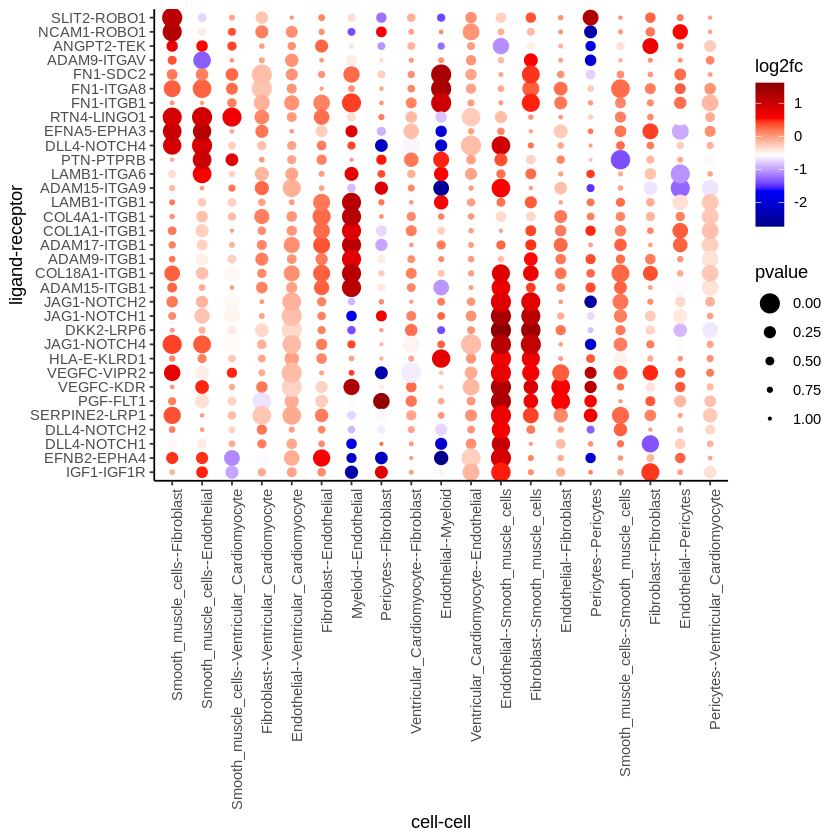
plotCCcomDotplot(gobject = my_giotto_object,
                 comScores = spatial_all_scores,
                 selected_LR = top_LR_ints,
                 selected_cell_LR = top_LR_cell_ints,
                 cluster_on = 'PI')

[ ]:
selected_spat = spatial_all_scores[p.adj <= 0.25 & abs(log2fc) > 0.1 & lig_nr >= 5 & rec_nr >= 5 & lig_expr > 0.5 & rec_expr > 0.5]
# selected_spat = spatial_all_scores[p.adj <= 0.1 & abs(log2fc) > 0.1 & lig_nr >= 5 & rec_nr >= 5 & LR_comb == 'JAG1-NOTCH2']
data.table::setorder(selected_spat, -PI)
[12]:
spatial_all_scores[(ligand == 'SLIT3') & (receptor == 'ROBO1')]
| LR_comb | lig_cell_type | lig_expr | ligand | rec_cell_type | rec_expr | receptor | LR_expr | lig_nr | rec_nr | rand_expr | av_diff | log2fc | pvalue | LR_cell_comb | p.adj | PI |
|---|---|---|---|---|---|---|---|---|---|---|---|---|---|---|---|---|
| <chr> | <fct> | <dbl> | <chr> | <fct> | <dbl> | <chr> | <dbl> | <int> | <int> | <dbl> | <dbl> | <dbl> | <dbl> | <chr> | <dbl> | <dbl> |
[127]:
## select top LR ##
selected_spat = spatial_all_scores[p.adj <= 0.25 & abs(log2fc) > 0.1 & lig_nr > 10 & rec_nr > 10 & lig_expr > 0.5 & rec_expr > 0.5]
# selected_spat = spatial_all_scores[p.adj <= 0.5 & abs(log2fc) > 0.1 & lig_nr >= 10 & rec_nr >= 10]
data.table::setorder(selected_spat, -PI)

top_LR_ints = unique(selected_spat[order(-abs(PI))]$LR_comb)[1:30]
top_LR_cell_ints = unique(selected_spat[order(-abs(PI))]$LR_cell_comb)[1:30]

plotCCcomHeatmap(gobject = my_giotto_object,
                 comScores = spatial_all_scores,
                 selected_LR = top_LR_ints,
                 selected_cell_LR = top_LR_cell_ints,
                 show = 'LR_expr')

[148]:
gobject = my_giotto_object
# comScores = spatial_all_scores
comScores = selected_spat
selected_LR = top_LR_ints
selected_cell_LR = top_LR_cell_ints
show_LR_names = TRUE
show_cell_LR_names = TRUE
cluster_on = c('PI', 'LR_expr', 'log2fc')
cor_method = c("pearson", "kendall", "spearman")
aggl_method = c("ward.D", "ward.D2", "single", "complete", "average", "mcquitty", "median", "centroid")
show_plot = NA
return_plot = NA
save_plot = NA
save_param =  list()
default_save_name = 'plotCCcomDotplot'
[149]:
dt_to_matrix <- function(x) {
  rownames = as.character(x[[1]])
  mat = methods::as(Matrix::as.matrix(x[,-1]), 'Matrix')
  rownames(mat) = rownames
  return(mat)
}

cor_giotto = function(x, ...) {
  x = as.matrix(x)
  return(stats::cor(x, ...))
}

t_giotto = function(mymatrix) {

  if(methods::is(mymatrix, 'dgCMatrix')) {
    return(Matrix::t(mymatrix)) # replace with sparseMatrixStats
  } else if(methods::is(mymatrix, 'Matrix')) {
    return(Matrix::t(mymatrix))
  } else {
    mymatrix = as.matrix(mymatrix)
    mymatrix = base::t(mymatrix)
    return(mymatrix)
  }
}
[150]:
cor_method = 'pearson'
aggl_method = 'ward.D'
selDT = comScores[LR_comb %in% selected_LR & LR_cell_comb %in% selected_cell_LR]

cluster_on = 'PI'
selDT_d = data.table::dcast.data.table(selDT, LR_cell_comb~LR_comb, value.var = cluster_on, fill = 0)
selDT_m = dt_to_matrix(selDT_d)

# remove zero variance
sd_rows = apply(selDT_m, 1, sd)
sd_rows_zero = names(sd_rows[sd_rows == 0])
if(length(sd_rows_zero) > 0) selDT_m = selDT_m[!rownames(selDT_m) %in% sd_rows_zero, ]

sd_cols = apply(selDT_m, 2, sd)
sd_cols_zero = names(sd_cols[sd_cols == 0])
if(length(sd_cols_zero) > 0) selDT_m = selDT_m[, !colnames(selDT_m) %in% sd_cols_zero]

## cells
corclus_cells_dist = stats::as.dist(1-cor_giotto(x = t_giotto(selDT_m), method = cor_method))
hclusters_cells = stats::hclust(d = corclus_cells_dist, method = aggl_method)
# clus_names = rownames(selDT_m)
# names(clus_names) = 1:length(clus_names)
# # clus_sort_names = clus_names[hclusters_cells$order]
# clus_sort_names = clus_names[order(clus_names)]

##############################################
# reorder cells
clus_names = rownames(selDT_m)
split_clus_names = strsplit(clus_names, split = "--")
clus_names_R = c(split_clus_names[[1]][2])
clus_names_L = c(split_clus_names[[1]][1])
for (i in 2:length(clus_names)){
    clus_names_R = c(clus_names_R, split_clus_names[[i]][2])
    clus_names_L = c(clus_names_L, split_clus_names[[i]][1])
    }

clus_names_L_reorder = clus_names_L[order(clus_names_R)]
clus_names_R_reorder = clus_names_R[order(clus_names_R)]
clus_names_reorderR = clus_names[order(clus_names_R)]


Receptors = unique(clus_names_R[order(clus_names_R)])
clus_names_reorder = c(clus_names_reorderR[clus_names_R[order(clus_names_R)] == Receptors[1]][order(clus_names_L_reorder[clus_names_R[order(clus_names_R)] == Receptors[1]])])
for (i in 2:length(Receptors)){
    clus_names_reorder = c(clus_names_reorder, clus_names_reorderR[clus_names_R[order(clus_names_R)] == Receptors[i]][order(clus_names_L_reorder[clus_names_R[order(clus_names_R)] == Receptors[i]])])
    }
clus_sort_names = clus_names_reorder
##############################################
selDT[, LR_cell_comb := factor(LR_cell_comb, clus_sort_names)]


## genes
corclus_genes_dist = stats::as.dist(1-cor_giotto(x = selDT_m, method = cor_method))
hclusters_genes = stats::hclust(d = corclus_genes_dist, method = aggl_method)
clus_names = colnames(selDT_m)
names(clus_names) = 1:length(clus_names)
clus_sort_names = clus_names[hclusters_genes$order]
selDT[, LR_comb := factor(LR_comb, clus_sort_names)]

pl = ggplot2::ggplot()
pl = pl + ggplot2::geom_point(data = selDT, ggplot2::aes_string(x = 'LR_cell_comb',
                                             y = 'LR_comb', size = 'pvalue', color = 'log2fc'))
pl = pl + ggplot2::theme_classic()
if(show_LR_names == TRUE) pl = pl + ggplot2::theme(axis.text.y = ggplot2::element_text(),
                                         axis.ticks.y = ggplot2::element_line())
if(show_cell_LR_names == TRUE) pl = pl + ggplot2::theme(axis.text.x = ggplot2::element_text(angle = 90, vjust = 1, hjust = 1),
                                              axis.ticks.x = ggplot2::element_line())
pl = pl + ggplot2::scale_fill_gradientn(colours = c('darkblue', 'blue', 'white', 'red', 'darkred'))
pl = pl + ggplot2::scale_size_continuous(range = c(3, 0.5)) + ggplot2::scale_color_gradientn(colours = c('darkblue', 'blue', 'white', 'red', 'darkred'))
pl = pl + ggplot2::labs(x = 'cell-cell', y = 'ligand-receptor')


# # print, return and save parameters
# show_plot = ifelse(is.na(show_plot), readGiottoInstructions(gobject, param = 'show_plot'), show_plot)
# save_plot = ifelse(is.na(save_plot), readGiottoInstructions(gobject, param = 'save_plot'), save_plot)
# return_plot = ifelse(is.na(return_plot), readGiottoInstructions(gobject, param = 'return_plot'), return_plot)
print(pl)
## print plot
# if(show_plot == TRUE) {
# print(pl)
# }
[151]:
# write.csv(selDT, '/home/share/xwanaf/sour_sep/newCKPT/MerM/giotto_data/selDT.csv', row.names = FALSE)
[152]:
# pl = ggplot2::ggplot()
# pl = pl + ggplot2::geom_point(data = selDT, ggplot2::aes_string(x = 'LR_cell_comb',
#                                              y = 'LR_comb', size = 'pvalue', color = 'log2fc'))
# options(repr.plot.width = 8, repr.plot.height = 10)
# pl = pl + ggplot2::theme_classic()
# if(show_LR_names == TRUE) pl = pl + ggplot2::theme(axis.text.y = ggplot2::element_text(),
#                                          axis.ticks.y = ggplot2::element_line())
# if(show_cell_LR_names == TRUE) pl = pl + ggplot2::theme(axis.text.x = ggplot2::element_text(angle = 90, vjust = 1, hjust = 1),
#                                               axis.ticks.x = ggplot2::element_line())
# # pl = pl + ggplot2::scale_fill_gradientn(colours = c('darkblue', 'blue', 'white', 'red', 'darkred'))
# pl = pl + ggplot2::scale_fill_gradientn(colours = c('darkblue', 'blue', 'lightblue', 'white', 'red'))
# # pl = pl + ggplot2::scale_size_continuous(range = c(3, 0.5)) + ggplot2::scale_color_gradientn(colours = c('darkblue', 'blue', 'white', 'red', 'darkred'))
# pl = pl + ggplot2::scale_size_continuous(range = c(3, 0.5)) + ggplot2::scale_color_gradientn(colours = c('darkblue', 'blue', 'lightblue', 'white', 'red'))

# pl = pl + ggplot2::labs(x = 'cell-cell', y = 'ligand-receptor')

# print(pl)
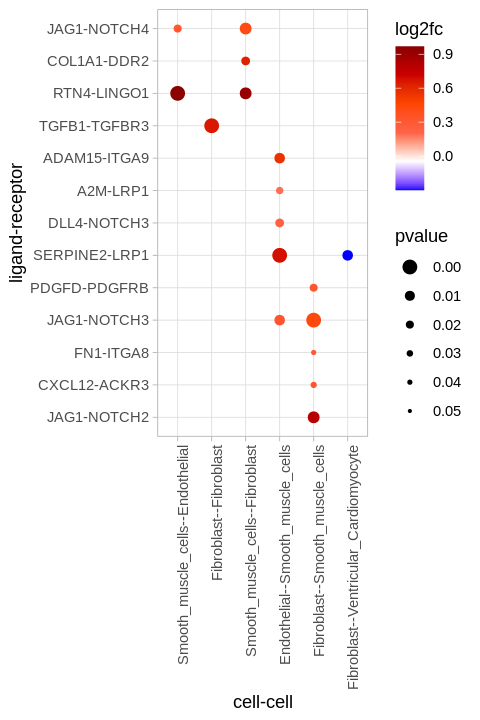
[153]:
pl = ggplot2::ggplot()
# pl = pl + ggplot2::geom_point(data = selDT, ggplot2::aes_string(x = 'LR_cell_comb',
#                                              y = 'LR_comb', size = 'pvalue', color = 'log2fc'))
pl = pl + ggplot2::geom_point(data = selDT, ggplot2::aes_string(x = 'LR_cell_comb',
                                             y = 'LR_comb', size = 'p.adj', color = 'log2fc'))
options(repr.plot.width = 4, repr.plot.height = 5)
pl = pl + ggplot2::theme_classic()
if(show_LR_names == TRUE) pl = pl + ggplot2::theme(axis.text.y = ggplot2::element_text(),
                                         axis.ticks.y = ggplot2::element_line())
if(show_cell_LR_names == TRUE) pl = pl + ggplot2::theme(axis.text.x = ggplot2::element_text(angle = 90, vjust = 1, hjust = 1),
                                              axis.ticks.x = ggplot2::element_line())
# pl = pl + ggplot2::scale_fill_gradientn(colours = c('darkblue', 'blue', 'white', 'red', 'darkred'))
# pl = pl + ggplot2::scale_fill_gradientn(colours = c('darkblue', 'blue', 'lightblue', 'white', 'red'))
# pl = pl + ggplot2::scale_fill_gradientn(colours = c('darkblue', 'blue', 'white', 'red'))
pl = pl + ggplot2::scale_fill_gradientn(colours = c('white', 'lightsalmon', 'red', 'darkred'))
pl = pl + ggplot2::scale_color_gradientn(colours=c('darkblue','blue', 'white', 'red','darkred'))
# pl = pl + ggplot2::scale_size_continuous(range = c(3, 0.5)) + ggplot2::scale_color_gradientn(colours = c('darkblue', 'blue', 'white', 'red', 'darkred'))
# pl = pl + ggplot2::scale_size_continuous(range = c(3, 0.1), limits = c(0, 0.2)) + ggplot2::scale_color_gradientn(colours = c('darkblue', 'blue', 'white', 'red'))
pl = pl + ggplot2::scale_size_continuous(range = c(3, 0.1), limits = c(0, 0.2)) + ggplot2::scale_color_gradientn(colours = c('white', 'lightsalmon', 'red', 'darkred'))

pl = pl + ggplot2::labs(x = 'cell-cell', y = 'ligand-receptor')

print(pl)
Scale for 'colour' is already present. Adding another scale for 'colour',
which will replace the existing scale.
[ ]:
[154]:
pl = ggplot2::ggplot()
# pl = pl + ggplot2::geom_point(data = selDT, ggplot2::aes_string(x = 'LR_cell_comb',
#                                              y = 'LR_comb', size = 'pvalue', color = 'log2fc'))
pl = pl + ggplot2::geom_point(data = selDT, ggplot2::aes_string(x = 'LR_cell_comb',
                                             y = 'LR_comb', size = 'p.adj', color = 'log2fc'))
options(repr.plot.width = 4, repr.plot.height = 5)
pl = pl + ggplot2::theme_classic()
if(show_LR_names == TRUE) pl = pl + ggplot2::theme(axis.text.y = ggplot2::element_text(),
                                         axis.ticks.y = ggplot2::element_line())
if(show_cell_LR_names == TRUE) pl = pl + ggplot2::theme(axis.text.x = ggplot2::element_text(angle = 90, vjust = 1, hjust = 1),
                                              axis.ticks.x = ggplot2::element_line())
# pl = pl + ggplot2::scale_fill_gradientn(colours = c('darkblue', 'blue', 'white', 'red', 'darkred'))
# pl = pl + ggplot2::scale_fill_gradientn(colours = c('darkblue', 'blue', 'lightblue', 'white', 'red'))
# pl = pl + ggplot2::scale_fill_gradientn(colours = c('darkblue', 'blue', 'white', 'red'))
pl = pl + ggplot2::scale_fill_gradientn(colours = c('white', 'lightsalmon', 'red', 'darkred'))
pl = pl + ggplot2::scale_color_gradientn(colours=c('darkblue','blue', 'white', 'red','darkred'))
# pl = pl + ggplot2::scale_size_continuous(range = c(3, 0.5)) + ggplot2::scale_color_gradientn(colours = c('darkblue', 'blue', 'white', 'red', 'darkred'))
# pl = pl + ggplot2::scale_size_continuous(range = c(3, 0.1), limits = c(0, 0.2)) + ggplot2::scale_color_gradientn(colours = c('darkblue', 'blue', 'white', 'red'))
pl = pl + ggplot2::scale_size_continuous(range = c(3, 0.1), limits = c(0, 0.2)) + ggplot2::scale_color_gradientn(colours = c('white', 'lightsalmon', 'red', 'darkred'))

pl = pl + ggplot2::labs(x = 'cell-cell', y = 'ligand-receptor')

print(pl)
Scale for 'colour' is already present. Adding another scale for 'colour',
which will replace the existing scale.

[155]:
# array(['Endothelial', 'Fibroblast', 'Lymphoid', 'Myeloid', 'Neuronal',
#        'Pericytes', 'Smooth_muscle_cells', 'Ventricular_Cardiomyocyte'],
#       dtype=object)
[156]:
selDT[(selDT$lig_cell_type == 'Myeloid') & (selDT$rec_cell_type == 'Endothelial')]
| LR_comb | lig_cell_type | lig_expr | ligand | rec_cell_type | rec_expr | receptor | LR_expr | lig_nr | rec_nr | rand_expr | av_diff | log2fc | pvalue | LR_cell_comb | p.adj | PI |
|---|---|---|---|---|---|---|---|---|---|---|---|---|---|---|---|---|
| <fct> | <fct> | <dbl> | <chr> | <fct> | <dbl> | <chr> | <dbl> | <int> | <int> | <dbl> | <dbl> | <dbl> | <dbl> | <fct> | <dbl> | <dbl> |
[157]:
selDT[(selDT$lig_cell_type == 'Endothelial') & (selDT$rec_cell_type == 'Smooth_muscle_cells')]
| LR_comb | lig_cell_type | lig_expr | ligand | rec_cell_type | rec_expr | receptor | LR_expr | lig_nr | rec_nr | rand_expr | av_diff | log2fc | pvalue | LR_cell_comb | p.adj | PI |
|---|---|---|---|---|---|---|---|---|---|---|---|---|---|---|---|---|
| <fct> | <fct> | <dbl> | <chr> | <fct> | <dbl> | <chr> | <dbl> | <int> | <int> | <dbl> | <dbl> | <dbl> | <dbl> | <fct> | <dbl> | <dbl> |
| SERPINE2-LRP1 | Endothelial | 0.8821606 | SERPINE2 | Smooth_muscle_cells | 0.7238008 | LRP1 | 1.605961 | 45 | 41 | 0.9649785 | 0.6409829 | 0.6797607 | 0.000 | Endothelial--Smooth_muscle_cells | 0.00000000 | 1.3056971 |
| ADAM15-ITGA9 | Endothelial | 0.9791948 | ADAM15 | Smooth_muscle_cells | 0.5732272 | ITGA9 | 1.552422 | 45 | 41 | 1.0205055 | 0.5319165 | 0.5604324 | 0.008 | Endothelial--Smooth_muscle_cells | 0.03600000 | 0.8090949 |
| JAG1-NOTCH3 | Endothelial | 1.1053646 | JAG1 | Smooth_muscle_cells | 2.2582759 | NOTCH3 | 3.363640 | 45 | 41 | 2.6518967 | 0.7117437 | 0.3318628 | 0.008 | Endothelial--Smooth_muscle_cells | 0.03600000 | 0.4791095 |
| DLL4-NOTCH3 | Endothelial | 0.8002950 | DLL4 | Smooth_muscle_cells | 2.2582759 | NOTCH3 | 3.058571 | 45 | 41 | 2.5862808 | 0.4722900 | 0.2336618 | 0.016 | Endothelial--Smooth_muscle_cells | 0.05760000 | 0.2896419 |
| A2M-LRP1 | Endothelial | 3.8846267 | A2M | Smooth_muscle_cells | 0.7238008 | LRP1 | 4.608427 | 45 | 41 | 4.0209976 | 0.5874298 | 0.1922517 | 0.024 | Endothelial--Smooth_muscle_cells | 0.08228571 | 0.2085307 |
| PDGFD-PDGFRB | Endothelial | 1.0304364 | PDGFD | Smooth_muscle_cells | 2.5353614 | PDGFRB | 3.565798 | 45 | 41 | 3.0924062 | 0.4733917 | 0.1994830 | 0.052 | Endothelial--Smooth_muscle_cells | 0.16904348 | 0.1540012 |
[158]:
min(selDT$log2fc)
-0.232504898981321
[165]:
selDT[log2fc == min(selDT$log2fc)]$log2fc = -0.3
[167]:
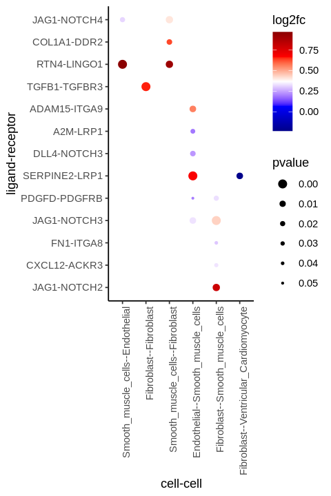
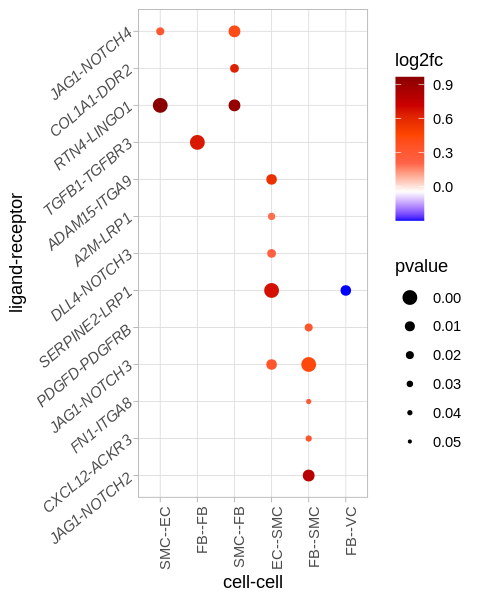
selDT
| LR_comb | lig_cell_type | lig_expr | ligand | rec_cell_type | rec_expr | receptor | LR_expr | lig_nr | rec_nr | rand_expr | av_diff | log2fc | pvalue | LR_cell_comb | p.adj | PI |
|---|---|---|---|---|---|---|---|---|---|---|---|---|---|---|---|---|
| <fct> | <fct> | <dbl> | <chr> | <fct> | <dbl> | <chr> | <dbl> | <int> | <int> | <dbl> | <dbl> | <dbl> | <dbl> | <fct> | <dbl> | <dbl> |
| RTN4-LINGO1 | Smooth_muscle_cells | 0.8793521 | RTN4 | Endothelial | 1.5048799 | LINGO1 | 2.384232 | 41 | 45 | 1.1699542 | 1.2142778 | 0.9680234 | 0.000 | Smooth_muscle_cells--Endothelial | 0.00000000 | 1.8593976 |
| SERPINE2-LRP1 | Endothelial | 0.8821606 | SERPINE2 | Smooth_muscle_cells | 0.7238008 | LRP1 | 1.605961 | 45 | 41 | 0.9649785 | 0.6409829 | 0.6797607 | 0.000 | Endothelial--Smooth_muscle_cells | 0.00000000 | 1.3056971 |
| RTN4-LINGO1 | Smooth_muscle_cells | 1.0054810 | RTN4 | Fibroblast | 2.7735005 | LINGO1 | 3.778981 | 28 | 36 | 1.9467534 | 1.8322281 | 0.9223406 | 0.004 | Smooth_muscle_cells--Fibroblast | 0.07200000 | 1.0539286 |
| JAG1-NOTCH2 | Fibroblast | 1.0529821 | JAG1 | Smooth_muscle_cells | 0.5056152 | NOTCH2 | 1.558597 | 36 | 28 | 0.8531829 | 0.7054145 | 0.7991388 | 0.004 | Fibroblast--Smooth_muscle_cells | 0.05760000 | 0.9905944 |
| ADAM15-ITGA9 | Endothelial | 0.9791948 | ADAM15 | Smooth_muscle_cells | 0.5732272 | ITGA9 | 1.552422 | 45 | 41 | 1.0205055 | 0.5319165 | 0.5604324 | 0.008 | Endothelial--Smooth_muscle_cells | 0.03600000 | 0.8090949 |
| JAG1-NOTCH3 | Fibroblast | 1.0529821 | JAG1 | Smooth_muscle_cells | 2.5971751 | NOTCH3 | 3.650157 | 36 | 28 | 2.6666231 | 0.9835341 | 0.4388250 | 0.000 | Fibroblast--Smooth_muscle_cells | 0.00000000 | 0.5787043 |
| COL1A1-DDR2 | Smooth_muscle_cells | 0.5387743 | COL1A1 | Fibroblast | 1.6158163 | DDR2 | 2.154591 | 28 | 36 | 1.3582296 | 0.7963610 | 0.6286476 | 0.016 | Smooth_muscle_cells--Fibroblast | 0.16457143 | 0.4926369 |
| JAG1-NOTCH3 | Endothelial | 1.1053646 | JAG1 | Smooth_muscle_cells | 2.2582759 | NOTCH3 | 3.363640 | 45 | 41 | 2.6518967 | 0.7117437 | 0.3318628 | 0.008 | Endothelial--Smooth_muscle_cells | 0.03600000 | 0.4791095 |
| JAG1-NOTCH4 | Smooth_muscle_cells | 2.1747544 | JAG1 | Fibroblast | 0.8322134 | NOTCH4 | 3.006968 | 28 | 36 | 2.2420046 | 0.7649631 | 0.4077633 | 0.004 | Smooth_muscle_cells--Fibroblast | 0.07200000 | 0.4659379 |
| DLL4-NOTCH3 | Endothelial | 0.8002950 | DLL4 | Smooth_muscle_cells | 2.2582759 | NOTCH3 | 3.058571 | 45 | 41 | 2.5862808 | 0.4722900 | 0.2336618 | 0.016 | Endothelial--Smooth_muscle_cells | 0.05760000 | 0.2896419 |
| PDGFD-PDGFRB | Fibroblast | 1.4379348 | PDGFD | Smooth_muscle_cells | 2.8907387 | PDGFRB | 4.328673 | 36 | 28 | 3.4314257 | 0.8972478 | 0.3266239 | 0.020 | Fibroblast--Smooth_muscle_cells | 0.13090909 | 0.2884188 |
| TGFB1-TGFBR3 | Fibroblast | 0.5620250 | TGFB1 | Fibroblast | 1.0270834 | TGFBR3 | 1.589108 | 53 | 53 | 0.9698985 | 0.6192100 | 0.6587881 | 0.000 | Fibroblast--Fibroblast | 0.00000000 | 0.2738376 |
| JAG1-NOTCH4 | Smooth_muscle_cells | 1.7198625 | JAG1 | Endothelial | 1.5427746 | NOTCH4 | 3.262637 | 41 | 45 | 2.6032133 | 0.6594238 | 0.3149177 | 0.020 | Smooth_muscle_cells--Endothelial | 0.16000000 | 0.2506367 |
| CXCL12-ACKR3 | Fibroblast | 0.6903565 | CXCL12 | Smooth_muscle_cells | 1.7590382 | ACKR3 | 2.449395 | 36 | 28 | 1.9232764 | 0.5261183 | 0.3334613 | 0.032 | Fibroblast--Smooth_muscle_cells | 0.17723077 | 0.2505831 |
| FN1-ITGA8 | Fibroblast | 2.8233985 | FN1 | Smooth_muscle_cells | 1.9694344 | ITGA8 | 4.792833 | 36 | 28 | 3.8838746 | 0.9089583 | 0.2964978 | 0.040 | Fibroblast--Smooth_muscle_cells | 0.19200000 | 0.2124996 |
| A2M-LRP1 | Endothelial | 3.8846267 | A2M | Smooth_muscle_cells | 0.7238008 | LRP1 | 4.608427 | 45 | 41 | 4.0209976 | 0.5874298 | 0.1922517 | 0.024 | Endothelial--Smooth_muscle_cells | 0.08228571 | 0.2085307 |
| PDGFD-PDGFRB | Endothelial | 1.0304364 | PDGFD | Smooth_muscle_cells | 2.5353614 | PDGFRB | 3.565798 | 45 | 41 | 3.0924062 | 0.4733917 | 0.1994830 | 0.052 | Endothelial--Smooth_muscle_cells | 0.16904348 | 0.1540012 |
| SERPINE2-LRP1 | Fibroblast | 0.6770152 | SERPINE2 | Ventricular_Cardiomyocyte | 0.6589103 | LRP1 | 1.335925 | 83 | 178 | 1.5870302 | -0.2511047 | -0.3000000 | 0.008 | Fibroblast--Ventricular_Cardiomyocyte | 0.11520000 | -0.2182169 |
[166]:
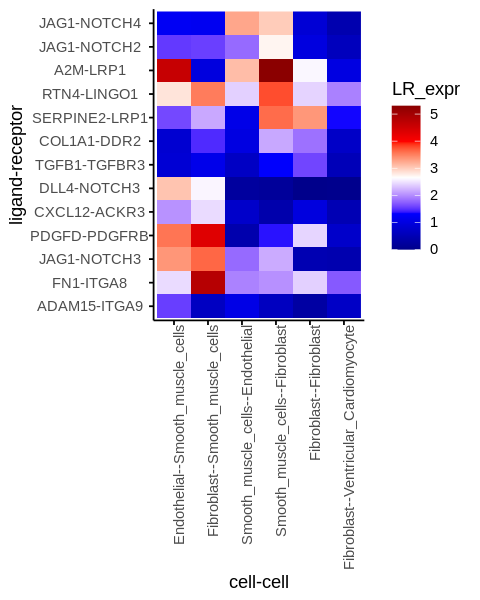
pl = ggplot2::ggplot()
pl = pl + ggplot2::geom_point(data = selDT, ggplot2::aes_string(x = 'LR_cell_comb',
                                             y = 'LR_comb', size = 'pvalue', color = 'log2fc'))
options(repr.plot.width = 4, repr.plot.height = 6)
pl = pl + ggplot2::theme_light()
if(show_LR_names == TRUE) pl = pl + ggplot2::theme(axis.text.y = ggplot2::element_text(),
                                         axis.ticks.y = ggplot2::element_line())
if(show_cell_LR_names == TRUE) pl = pl + ggplot2::theme(axis.text.x = ggplot2::element_text(angle = 90, vjust = 1, hjust = 1),
                                              axis.ticks.x = ggplot2::element_line())
#pl = pl + ggplot2::scale_color_gradient2(low="blue", mid="white", high="red")
pl = pl + ggplot2::scale_color_gradientn(colours=c('blue', 'white', 'tomato', 'orangered', 'red3', 'darkred'))
pl = pl + ggplot2::scale_size_continuous(range = c(3.5, 0.5), limits = c(0, 0.05))
pl = pl + ggplot2::labs(x = 'cell-cell', y = 'ligand-receptor')
print(pl)
Warning message:
“Removed 1 rows containing missing values (geom_point).”
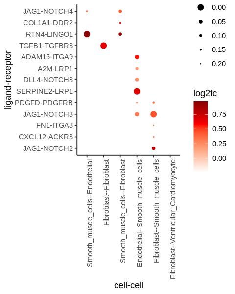
[184]:
pl = ggplot2::ggplot()
pl = pl + ggplot2::geom_point(data = selDT, ggplot2::aes_string(x = 'LR_cell_comb',
                                             y = 'LR_comb', size = 'pvalue', color = 'log2fc'))
options(repr.plot.width = 4, repr.plot.height = 5)
pl = pl + ggplot2::theme_light()
if(show_LR_names == TRUE) pl = pl + ggplot2::theme(axis.text.y = ggplot2::element_text(face="italic",angle=40),
                                         axis.ticks.y = ggplot2::element_line())
if(show_cell_LR_names == TRUE) pl = pl + ggplot2::theme(axis.text.x = ggplot2::element_text(angle = 90, vjust = 1, hjust = 1),
                                              axis.ticks.x = ggplot2::element_line())
#pl = pl + ggplot2::scale_color_gradient2(low="blue", mid="white", high="red")
pl = pl + ggplot2::scale_color_gradientn(colours=c('blue', 'white', 'tomato', 'orangered', 'red3', 'darkred'))
pl = pl + ggplot2::scale_size_continuous(range = c(3.5, 0.5), limits = c(0, 0.05))
pl = pl + ggplot2::labs(x = 'cell-cell', y = 'ligand-receptor')
pl = pl + ggplot2::scale_x_discrete(labels=c("Smooth_muscle_cells--Endothelial" = "SMC--EC",
                                            "Endothelial--Smooth_muscle_cells" = "EC--SMC",
                                            "Smooth_muscle_cells--Fibroblast" = "SMC--FB",
                                            "Fibroblast--Smooth_muscle_cells" = "FB--SMC",
                                            "Fibroblast--Fibroblast" = "FB--FB",
                                            "Fibroblast--Ventricular_Cardiomyocyte" = "FB--VC"))
print(pl)
Warning message:
“Removed 1 rows containing missing values (geom_point).”
[176]:
selDT
| LR_comb | lig_cell_type | lig_expr | ligand | rec_cell_type | rec_expr | receptor | LR_expr | lig_nr | rec_nr | rand_expr | av_diff | log2fc | pvalue | LR_cell_comb | p.adj | PI |
|---|---|---|---|---|---|---|---|---|---|---|---|---|---|---|---|---|
| <fct> | <fct> | <dbl> | <chr> | <fct> | <dbl> | <chr> | <dbl> | <int> | <int> | <dbl> | <dbl> | <dbl> | <dbl> | <fct> | <dbl> | <dbl> |
| RTN4-LINGO1 | Smooth_muscle_cells | 0.8793521 | RTN4 | Endothelial | 1.5048799 | LINGO1 | 2.384232 | 41 | 45 | 1.1699542 | 1.2142778 | 0.9680234 | 0.000 | Smooth_muscle_cells--Endothelial | 0.00000000 | 1.8593976 |
| SERPINE2-LRP1 | Endothelial | 0.8821606 | SERPINE2 | Smooth_muscle_cells | 0.7238008 | LRP1 | 1.605961 | 45 | 41 | 0.9649785 | 0.6409829 | 0.6797607 | 0.000 | Endothelial--Smooth_muscle_cells | 0.00000000 | 1.3056971 |
| RTN4-LINGO1 | Smooth_muscle_cells | 1.0054810 | RTN4 | Fibroblast | 2.7735005 | LINGO1 | 3.778981 | 28 | 36 | 1.9467534 | 1.8322281 | 0.9223406 | 0.004 | Smooth_muscle_cells--Fibroblast | 0.07200000 | 1.0539286 |
| JAG1-NOTCH2 | Fibroblast | 1.0529821 | JAG1 | Smooth_muscle_cells | 0.5056152 | NOTCH2 | 1.558597 | 36 | 28 | 0.8531829 | 0.7054145 | 0.7991388 | 0.004 | Fibroblast--Smooth_muscle_cells | 0.05760000 | 0.9905944 |
| ADAM15-ITGA9 | Endothelial | 0.9791948 | ADAM15 | Smooth_muscle_cells | 0.5732272 | ITGA9 | 1.552422 | 45 | 41 | 1.0205055 | 0.5319165 | 0.5604324 | 0.008 | Endothelial--Smooth_muscle_cells | 0.03600000 | 0.8090949 |
| JAG1-NOTCH3 | Fibroblast | 1.0529821 | JAG1 | Smooth_muscle_cells | 2.5971751 | NOTCH3 | 3.650157 | 36 | 28 | 2.6666231 | 0.9835341 | 0.4388250 | 0.000 | Fibroblast--Smooth_muscle_cells | 0.00000000 | 0.5787043 |
| COL1A1-DDR2 | Smooth_muscle_cells | 0.5387743 | COL1A1 | Fibroblast | 1.6158163 | DDR2 | 2.154591 | 28 | 36 | 1.3582296 | 0.7963610 | 0.6286476 | 0.016 | Smooth_muscle_cells--Fibroblast | 0.16457143 | 0.4926369 |
| JAG1-NOTCH3 | Endothelial | 1.1053646 | JAG1 | Smooth_muscle_cells | 2.2582759 | NOTCH3 | 3.363640 | 45 | 41 | 2.6518967 | 0.7117437 | 0.3318628 | 0.008 | Endothelial--Smooth_muscle_cells | 0.03600000 | 0.4791095 |
| JAG1-NOTCH4 | Smooth_muscle_cells | 2.1747544 | JAG1 | Fibroblast | 0.8322134 | NOTCH4 | 3.006968 | 28 | 36 | 2.2420046 | 0.7649631 | 0.4077633 | 0.004 | Smooth_muscle_cells--Fibroblast | 0.07200000 | 0.4659379 |
| DLL4-NOTCH3 | Endothelial | 0.8002950 | DLL4 | Smooth_muscle_cells | 2.2582759 | NOTCH3 | 3.058571 | 45 | 41 | 2.5862808 | 0.4722900 | 0.2336618 | 0.016 | Endothelial--Smooth_muscle_cells | 0.05760000 | 0.2896419 |
| PDGFD-PDGFRB | Fibroblast | 1.4379348 | PDGFD | Smooth_muscle_cells | 2.8907387 | PDGFRB | 4.328673 | 36 | 28 | 3.4314257 | 0.8972478 | 0.3266239 | 0.020 | Fibroblast--Smooth_muscle_cells | 0.13090909 | 0.2884188 |
| TGFB1-TGFBR3 | Fibroblast | 0.5620250 | TGFB1 | Fibroblast | 1.0270834 | TGFBR3 | 1.589108 | 53 | 53 | 0.9698985 | 0.6192100 | 0.6587881 | 0.000 | Fibroblast--Fibroblast | 0.00000000 | 0.2738376 |
| JAG1-NOTCH4 | Smooth_muscle_cells | 1.7198625 | JAG1 | Endothelial | 1.5427746 | NOTCH4 | 3.262637 | 41 | 45 | 2.6032133 | 0.6594238 | 0.3149177 | 0.020 | Smooth_muscle_cells--Endothelial | 0.16000000 | 0.2506367 |
| CXCL12-ACKR3 | Fibroblast | 0.6903565 | CXCL12 | Smooth_muscle_cells | 1.7590382 | ACKR3 | 2.449395 | 36 | 28 | 1.9232764 | 0.5261183 | 0.3334613 | 0.032 | Fibroblast--Smooth_muscle_cells | 0.17723077 | 0.2505831 |
| FN1-ITGA8 | Fibroblast | 2.8233985 | FN1 | Smooth_muscle_cells | 1.9694344 | ITGA8 | 4.792833 | 36 | 28 | 3.8838746 | 0.9089583 | 0.2964978 | 0.040 | Fibroblast--Smooth_muscle_cells | 0.19200000 | 0.2124996 |
| A2M-LRP1 | Endothelial | 3.8846267 | A2M | Smooth_muscle_cells | 0.7238008 | LRP1 | 4.608427 | 45 | 41 | 4.0209976 | 0.5874298 | 0.1922517 | 0.024 | Endothelial--Smooth_muscle_cells | 0.08228571 | 0.2085307 |
| PDGFD-PDGFRB | Endothelial | 1.0304364 | PDGFD | Smooth_muscle_cells | 2.5353614 | PDGFRB | 3.565798 | 45 | 41 | 3.0924062 | 0.4733917 | 0.1994830 | 0.052 | Endothelial--Smooth_muscle_cells | 0.16904348 | 0.1540012 |
| SERPINE2-LRP1 | Fibroblast | 0.6770152 | SERPINE2 | Ventricular_Cardiomyocyte | 0.6589103 | LRP1 | 1.335925 | 83 | 178 | 1.5870302 | -0.2511047 | -0.3000000 | 0.008 | Fibroblast--Ventricular_Cardiomyocyte | 0.11520000 | -0.2182169 |
[ ]:
[144]:
pl = ggplot2::ggplot()
pl = pl + ggplot2::geom_point(data = selDT, ggplot2::aes_string(x = 'LR_cell_comb',
                                             y = 'LR_comb', size = 'p.adj', color = 'log2fc'))
options(repr.plot.width = 4, repr.plot.height = 6)
pl = pl + ggplot2::theme_light()
if(show_LR_names == TRUE) pl = pl + ggplot2::theme(axis.text.y = ggplot2::element_text(),
                                         axis.ticks.y = ggplot2::element_line())
if(show_cell_LR_names == TRUE) pl = pl + ggplot2::theme(axis.text.x = ggplot2::element_text(angle = 90, vjust = 1, hjust = 1),
                                              axis.ticks.x = ggplot2::element_line())
#pl = pl + ggplot2::scale_color_gradient2(low="blue", mid="white", high="red")
pl = pl + ggplot2::scale_color_gradientn(colours=c('blue', 'white', 'tomato', 'orangered', 'red3', 'darkred'))
pl = pl + ggplot2::scale_size_continuous(range = c(3.5, 0.9), limits = c(0, 0.2))
pl = pl + ggplot2::labs(x = 'cell-cell', y = 'ligand-receptor')
print(pl)

[ ]:
[ ]: